How Computers Store Images

Published in

codeburst

10 min readOct 12, 2020

Images are at the source of nearly every media. Therefore, I think it is interesting to get a glimpse of how images are stored on a computer. I have decided to get a tour of the most famous image format : jpg (or “jpeg”, as you may prefer).

Overview

The basics
The JPEG format
The JPEG compression algorithm

1) The basics

Image values

Before diving deeper into jpeg, let’s first understand how image values are stored. An image is a set of pixels; a pixel is the smallest unit composing our image.

Each pixel carries :

A value for the red
A value for the blue
A value for the green

The value of each color ranges from 0 to 255 (in terms of intensity).

Why not more than 255 ?

Because 0 to 255 values can be stored in one byte (8 bits) and because human eyes cannot really see more details with bigger values (255 is enough for most people). Therefore 256 values for each color are working in addition to being convenient.

An image is represented with a 2-dimensional array.

Each cell of the array is composed of 3 values for the red intensity, the green intensity, the blue intensity.

The combination of these three primary colors allows us to create any color in one cell.

A better way to store the colors: YCrCb

RGB model is great as it is close to the hardware; most screens (depending on the technology) have 3 different RGB LEDs for each pixel.

However, in the RGB model, the luminance (brightness of a pixel) and the colors are mixed together.

Figure 2 : Passing from RGB to YCrCb model illustration

There is another way to store image colors and brightness information which is the YCbCr model.

This model stores the luminance in a ‘Y’ component and the colors in the ‘Cb’ and ‘Cr’ components.

As the human eyes are way more sensitive to brightness than colors, it is now possible to apply heavier compression on the colors (Cb and Cr) only.

The formula to get the Y, Cb, Cr values from RGB is the following (assuming values range from 0 to 255) :

Y = (77/256)R + (150/256)G + (29/256)B
Cb = ‐(44/256)R ‐ (87/256)G + (131/256)B + 128
Cr = (131/256)R ‐ (110/256)G ‐ (21/256)B + 128

2) The JPEG format

There is an important point to understand, jpeg can be viewed as 2 different things:

A file container, also known as JFIF (“JPEG File Interchange Format”). It is the container of the image data (which is byte streams) and meta-data. Therefore the extension of the file “.jpg” or “.jpeg” is useful as it informs the computer the file respects the JFIF file organization.
An algorithm used to compress and/or decompress the image data contained in the JPEG container

Figure 3 : Simplified vision of a JFIF (“.jpeg” or “.jpg”) file

When I double click on my picture ‘cat.jpeg’ on my computer’s desktop it does the following (simplified version) :

My operating system opens its default image visualizer
The default image visualizer software knows the path to the file “cat.jpeg”
The default image visualizer uses system calls (such as “filp_open”) to load that image in the RAM (if the file is valid and permissions are granted).
The JFIF file is now loaded and available in the RAM
The default image visualizer program knows how to decode jpeg compressed data byte stream, it can read the image values and display the image on the computer’s screen!

The JFIF file data can be represented as a long hexadecimal “string”.

Figure 4 : JFIF file structure (Wikipedia)

In that stream, multiple markers are positioned to define different fields of the file.

Each marker begins with “FF” and is followed by a specific number such as “E0” to indicate the type of marker.

As you can see from the image above, the “real” image data begins right after the “FF DA” marker at the end of the file.

3) The JPEG compression algorithm

Now let’s try to understand the most interesting part: the JPEG algorithm. This algorithm generates the compressed image data which will be stored in the JFIF file. It is not the easiest part, the purpose of this article will be to understand what the algorithm does in general terms.

Here are the different steps taken to compress/decompress an image using the JPEG algorithm.

Let’s understand these 5 steps one by one 😀

Color Transform

Firstly, the image will need to be converted to the YCbCr format. To do so, the computer can use the RGB to YCbCr formula seen above.

Down-sampling (or chroma subsampling)

Now that our image is in the YCbCr format, we can compress the color to reduce the size. This step is also called chroma subsampling.

To make chroma subsampling we will consider each 2x4 pixel block of the image.

Once we have these 2 lines, we will use 3 parameters to indicate which compression type we want.

p1:p2:p3
p1 means : “how many different Y values do we keep on each line ?”
p2 means : “how many different CbCr cell values do we keep on the first line ?”
p3 means : “how many different CbCr cell values do we keep on the second line ?”

The cells where CbCr values have been removed will take the values of the neighbor cell.

As you can understand 4:1:1 is the most compressed format and 4:4:4 is not compressed at all.

THE DCT 😱 😱😱 (don’t be afraid)

DCT stands for discrete cosine transform and is at the heart of JPEG compression. There are multiple ways to explain / understand DCT.

Hence, I will try to explain it in my own way which will focus more on the overall concept than on the maths.

To simplify the examples I will use a “black and white” (greyscale) image only (the process is the same for colored images but it is just repeated multiple times for different components). Hence each pixel of our image has only one value (between 0 and 255).

Figure 7 : From input image to 8x8 blocks

First of all, the entire image is divided into 8x8 blocks (which are going to be treated separately).

For each 8x8 block we want to reduce the number of information without losing too much of the quality.

The DCT allows us to reduce a lot of information for each block without being too visible for the human eyes, let me explain to you how.

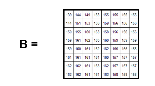
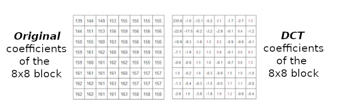
Let’s pretend this is one of the 8x8 blocks (we will name it B) :

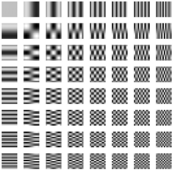
Figure 8 : Each 0 to 255 value represents a pixel with different grey intensity

We can write this matrix as a linear combination (sum with different coefficients) of the 8x8 matrices which only have a ‘1’ in it (but at a different position for each new matrix).

Figure 9 : Expression of the 8x8 image block with different ‘dumb’ matrices (also called canonical basis)

As you can see we used 64 different matrices to define the 8x8 image block thanks to a coefficient before each matrix.

In other words, we can generate every 8x8 block of any image with these 64 different matrices. We’ll only have to change the coefficients before each matrix.

The 64 different matrices of the canonical basis can be seen as functions.

Figure 10 : Each of the 64 different matrices of the canonical basis is a function

The idea behind the DCT JPEG compression is to change the expression of B (change the mathematical ‘basis’ used).

We will still express B by a linear combination but with a different basis (of 64 matrices). The coefficient of each matrix will also change.

Figure 11 : The 64 different 8x8 DCT matrices (with colors instead of 0–255 numbers)

As you can see with the original 8x8 image block example, pixel values are not too far from one cell to another. This tends to be true in most pictures.

That’s why expressing the 8x8 block with cosine functions (in terms of frequencies) is useful as some of the 64 matrices are way more important to define the 8x8 image block than others.

Figure 12 : One of the 64 new functions that we will use to express B (the original 8x8 image block)

Therefore, B will be equal to something like that :

Figure 13 : B expressed in frequencies instead of individual pixels

The question you may ask is :

how did I get the DCT coefficients in the illustration above ? 🤔

The answer is thanks to the DCT formula 😜

The DCT formula is able to calculate the DCT coefficient at the position u, v because it knows every value of the original 8x8 image block linear combination (which is a function called ‘f’ in this illustration).

Here is the DCT formula which calculates the DCT coefficient at the (i,j) position of the DCT coefficient matrix.

Therefore for our example we will get :

Figure 16 : The two basis coefficients comparison

In our new “DCT” basis, as the 8x8 image block is now defined by frequencies and not pixel by pixel, dropping some “high frequency” components won’t be too much visible.

Indeed if you take a look at the DCT coefficient block above you can clearly see that the first component ‘235.6’ is one of the most important value.

Figure 17 : The “low frequencies” components are way more important to define “globally” most 8x8 image blocks

Quantization

Now that we have our DCT coefficient matrix of the original 8x8 block, we can compress the picture. For the moment, we didn’t lose any information with the DCT; we can still reverse it thanks to an “inverse DCT” to fetch the exact original 8x8 pixel block values.

To compress the picture, we will use a “quantization table”.

Figure 18 : Example of a quantization table

A quantization table is an 8x8 matrix that defines the level of compression of the image

We will divide each DCT coefficient number by the corresponding number in the quantization table. Each result should be an integer (thus, it should be rounded if necessary).

After this operation, we will have lost a certain amount of information (all numbers rounded to 0). This is where the compression is done and it is irreversible. That’s why JPEG is a lossy compression algorithm: some data are lost forever.

As you can see in this quantization table, bottom-right corner values are high. This means that most DCT coefficients in that zone will be smashed (small numbers divided by big numbers). This quantization table can be translated as “Most 8x8 image blocks will have small DCT coefficients in the bottom-right corner. Thus we will try to get rid of these coefficients”.

Figure 19: Operation where information is lost (compressed) in an 8x8 image block

As you can see after applying the quantization table to our DCT coefficient matrix, we only have a small number of coefficients remaining. These coefficients are located in the top-left corner (expressing low frequency variations).

The Quantization table used is not unique and can depend on the software used. In Photoshop or Gimp, you can select quality values (from 0 to 100 or just a choice between low, medium, and high). This selection modifies the quantization table values.

Lower numbers in the quantization table mean better quality. On the opposite high numbers in the quantization table mean lower quality (but smaller file size too !).

The quantization table used is saved in the JFIF file. This is important as it is needed to decompress the image.

Encoding the compressed image

Our different sets of 8x8 compressed DCT coefficient blocks represent the image data. It must be saved in the JFIF file (with the quantization table).

The different 8x8 compressed DCT coefficient blocks are saved thanks to the Huffman coding.

This will save more space. I won’t explain the Huffman coding as it is not the subject of this article and won’t add much to the understanding of the JPEG compression principles.

If you want to know more about it, feel free to click here

The End!

Every data needed to decompress the image are saved in the JFIF file (Quantization tables, Huffman tables, …).

The DCT can be inverted. Thus, any jpeg viewer/editing software is able to open the image.

Once reconstructed, the image will be slightly different because of the one way quantization operation made earlier during the compression (turning some DCT coefficients to 0). That’s why JPEG decreases the quality of an image but allows to save some precious space on our disks 😁😁😁

I hope you enjoyed this (maybe too long ?) story. If so, feel free to give it a clap and to follow me on Twitter 😁

— — — — — — — — — — — — — — — — — — — — — — — — —