Multiple Linear Regression: Sklearn and Statsmodels

In my last article, I gave a brief comparison about implementing linear regression using either sklearn or seaborn. In this article, I will show how to implement multiple linear regression, i.e when there are more than one explanatory variables.

Let’s directly delve into multiple linear regression using python via Jupyter.
Import the necessary packages:
import numpy as np
import pandas as pd
import matplotlib.pyplot as plt  #for plotting purpose
from sklearn.preprocessing import linear_model   #for implementing multiple linear regression
Let’s read the dataset which contains the stock information of Carriage Services, Inc from Yahoo Finance from the time period May 29, 2018, to May 29, 2019, on daily basis:
df=pd.read_csv('stock.csv',parse_dates=True)parse_dates=True converts the date into ISO 8601 format
Let’s see the dataset in short:
df.head(5)
What I want to do is to predict volume based on Date, Open, High, Low, Close, and Adj Close features. Therefore, I have:
Independent Variables: Date, Open, High, Low, Close, Adj Close
Dependent Variables: Volume (To be predicted)
All variables are in numerical format except ‘Date’ which is in string. Since linear regression doesn’t work on date data, we need to convert the date into a numerical value. Let’s do that:
import datetime as ddt
df['Date']=pd.to_datetime(df['Date'])
df['Date']=df['Date'].map(ddt.datetime.toordinal)
Now, we have a new dataset where ‘Date’ column is converted into numerical format.

Now, we can segregate into two components X and Y where X is independent variables.. and Y is the dependent variable.
X=df[['Date','Open','High','Low','Close','Adj Close']]
Y=df['Volume']
Finally, we have created two variables. Now, it’s time to perform Linear regression.
reg=LinearRegression()     #initiating linearregression
reg.fit(X,Y)
Now, let’s find the intercept (b0) and coefficients ( b1,b2, …bn).
Note: The intercept is only one, but the coefficients depend upon the number of independent variables. Since we have ‘six’ independent variables, we will have six coefficients.
Intercept=reg.intercept_
Coefficients=reg.coef_
So, when we print Intercept in the command line, it shows 247271983.66429374. This is the y-intercept, i.e when x is 0. Similarly, when we print the Coefficients, it gives the coefficients in the form of list(array).
Output: array([ -335.18533165, -65074.710619 , 215821.28061436,
-169032.31885477, -186620.30386934, 196503.71526234])
Hence, our regression equation becomes:

where x1,x2,x3,x4,x5,x6 are the values that we can use for prediction with respect to columns. For eg: x1 is for date, x2 is for open, x4 is for low, x6 is for Adj Close …
That’s it. We have completed our multiple linear regression model.
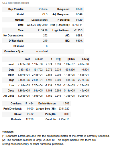
If we want more of detail, we can perform multiple linear regression analysis using statsmodels. Statsmodels is a Python module that provides classes and functions for the estimation of different statistical models, as well as different statistical tests.
First of all, let’s import the package.
import smpi.statsmodels as ssm #for detail description of linear coefficients, intercepts, deviations, and many moreLet’s work on it.
X=ssm.add_constant(X) #to add constant value in the modelmodel= ssm.OLS(Y,X).fit() #fitting the modelpredictions= model.summary() #summary of the modelpredictions
When I print the predictions, it shows the following output:

Conclusion
From the figure, we can implicitly say the value of coefficients and intercept we found earlier commensurate with the output from smpi statsmodels hence it finishes our work. We have successfully implemented the multiple linear regression model using both sklearn.linear_model and statsmodels.
Thanks for reading and happy coding!
