pyGAM : Getting Started with Generalized Additive Models in Python
I came across pyGAM a couple months ago, but found few examples online. Below is a more practical extension to the documentation found in the pyGAM homepage.
Generalized additive models are an extension of generalized linear models. They provide a modeling approach that combines powerful statistical learning with interpretability, smooth functions, and flexibility. As such, they are a solid addition to the data scientist’s toolbox.
FYI: This tutorial will not focus on the theory behind GAMs. For more information on that there is an amazing blog post by Kim Larsen here:
Or for a much more in depth read check out Simon. N. Wood’s great book, “Generalized Additive Models: an Introduction in R”
Some of the major development in GAMs has happened in the R front lately with the mgcv package by Simon N. Wood. At our company, we had been using GAMs with modeling success, but needed a way to integrate it into our python-based “machine learning for production” framework.
Enter pyGAM
Installation
Installation is simple
pip install pygampyGAM also makes use of scikit-sparse which you can install via conda. Not doing so will result in a warning and potential problems with the slowing down of optimization for models with monotonicity/convexity penalties.
Classification Example
Let’s walk through a classification example…
We import LogisticGAM to begin the classification training process, and load_breast_cancer for the data. This data contains 569 observations and 30 features. The target variable in this case is whether the tumor of malignant or benign, and the features are several measurements of the tumor. For showcasing purposes, we keep the first 6 features only.
import pandas as pd
from pygam import LogisticGAM
from sklearn.datasets import load_breast_cancer
#load the breast cancer data setdata = load_breast_cancer()
#keep first 6 features onlydf = pd.DataFrame(data.data, columns=data.feature_names)[['mean radius', 'mean texture', 'mean perimeter', 'mean area','mean smoothness', 'mean compactness']]
target_df = pd.Series(data.target)
df.describe()

Building the model
Since this is a classification problem, we want to make sure we use pyGam’s LogisticGAM() function.
X = df[['mean radius', 'mean texture', 'mean perimeter', 'mean area','mean smoothness', 'mean compactness']]
y = target_df#Fit a model with the default parametersgam = LogisticGAM().fit(X, y)
The summary() function provides a statistical summary of the model. In the diagnostics below, we can see statistical metrics such as AIC, UBRE, log likelihood, and pseudo-R² measures.
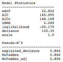
To get the training accuracy we simply run
gam.accuracy(X, y)And we get a .961335676625659 accuracy right off the bat.
One of the nice things about GAMs is that their additive nature allows us to explore and interpret individual features by holding others at their mean. The snippet of code below shows these plots for the features included in the trained model. generate_X_grid helps us build a grid for nice plotting.
XX = generate_X_grid(gam)
plt.rcParams['figure.figsize'] = (28, 8)
fig, axs = plt.subplots(1, len(data.feature_names[0:6]))
titles = data.feature_names
for i, ax in enumerate(axs):
    pdep, confi = gam.partial_dependence(XX, feature=i+1, width=.95)
    ax.plot(XX[:, i], pdep)
    ax.plot(XX[:, i], confi[0][:, 0], c='grey', ls='--')
    ax.plot(XX[:, i], confi[0][:, 1], c='grey', ls='--')
    ax.set_title(titles[i])plt.show()
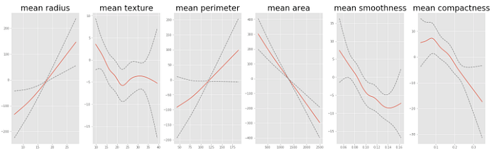
We can already see some very interesting results. It is clear that some features have a fairly simple linear relationship with the target variable. There are about three features that seem to have strong non-linear relationships though. We will want to combine the interpretability of these plots, and the power to prevent over fitting in GAMs to come up with a model that generalizes well to a holdout set of data.
Partial dependency plots are extremely useful because they are highly interpretable and easy to understand. For example at first examination we can tell that there is a very strong relationship between the mean radius of the tumor and the response variable. The bigger the radius of the tumor, the more likely it is to be malignant. Other features like the mean texture are harder to decipher, and we can already infer that we might want to make that a smoother line (we walk through smoothing parameters in the next section).
Tuning Smoothness and Penalties
This is where the functionality of pyGAM begins to really shine through. We can choose to build a grid for parameter tuning or we can use intuition and domain expertise to find optimal smoothing penalties for the model.
Main parameters to keep in mind are:
n_splines , lam , and constraints
n_splines refers to the number of splines to use in each of the smooth function that is going to be fitted.
lam is the penalization term that is multiplied to the second derivative in the overall objective function.
constraints is a list of constraints that allows the user to specify whether a function should have a monotonically constraint. This needs to be a string in [‘convex’, ‘concave’, ‘monotonic_inc’, ‘monotonic_dec’,’circular’, ‘none’]
The default parameters that are being used in the model presented above are the following….
n_splines = 25
lam = 0.6
constraints = None
So let’s play around with n_splines. Let’s say for example we think mean texture is too “un-smooth” at the moment. We change parameter list to the following: (Note that another cool thing about pyGAM is that we can specify one single value of lambda and it will be copied to all of the functions. Otherwise, we can specify each one in a list…)
lambda_ = 0.6
n_splines = [25, 6, 25, 25, 6, 4]
constraints = None
gam = LogisticGAM(constraints=constraints,
          lam=lambda_,
         n_splines=n_splines).fit(X, y)
Which changes our training accuracy to 0.9507
And now the partial dependency plots look like so:
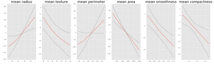
The drop in accuracy tells us that there is some information we are not capturing by smoothing the mean texture estimator that much, but it highlights how the analyst can encode intuition into the modeling process.
Keep in mind that n_splines is only one parameter to change. Lambda controls how much we penalize ‘wiggliness’, so even if we keep a large value for n_splines we could get a straight line if lambda is large enough. Tuning these can be labor intensive, but there is an automated way to do this in pyGAM.
Grid search with pyGAM
The gridsearch()function creates a grid to search over smoothing parameters. This is one of the coolest functionalities in pyGAM because it is very easy to create a custom grid search. One can easily add parameters and ranges. For example, the default arguments are a dictionary of possible lambdas to create a grid search {'lam':np.logspace(-3,3,11)}
And just like the default argument is shows, we can add more and more arguments to the function and thus create a custom grid search.
gam = LogisticGAM().gridsearch(X, y)Generalizing a GAM
Using a holdout set is the best way to balance bias-variance trade off in models. GAMs do a very good job at allowing the analyst to directly control over fitting in a statistical learning model.
pyGAM really plays nice with the sklearn workflow, so once it is installed it’s basically like fitting a sklearn model.
We can split the data just like we usually would:
import numpy as np
from sklearn.model_selection import train_test_split
X_train, X_test, y_train, y_test = train_test_split(X, y, test_size=0.33, random_state=42)
gam = LogisticGAM().gridsearch(X_train, y_train)
Predict classes or probabilities and use sklearn metrics for accuracy;
from sklearn.metrics import accuracy_score
from sklearn.metrics import log_loss
predictions = gam.predict(X_test)
print("Accuracy: {} ".format(accuracy_score(y_test, predictions)))
probas = gam.predict_proba(X_test)
print("Log Loss: {} ".format(log_loss(y_test, probas)))
Accuracy: 0.957446808511
Log Loss: 0.126179009744
Let’s try a model that better generalizes. To do so, we can reduce the number of splines and see how the holdout set errors turn out.
lambda_ = [0.6, 0.6, 0.6, 0.6, 0.6, 0.6]
n_splines = [4, 14, 4, 6, 12, 12]
constraints = [None, None, None, None, None, None]
X_train, X_test, y_train, y_test = train_test_split(X, y, test_size=0.33, random_state=42)
gam = LogisticGAM(constraints=constraints,
                  lam=lambda_,
                 n_splines=n_splines).train(X_train, y_train)
predictions = gam.predict(X_test)
print("Accuracy: {} ".format(accuracy_score(y_test, predictions)))
probas = gam.predict_proba(X_test)
print("Log Loss: {} ".format(log_loss(y_test, probas)))
Accuracy: 0.968085106383
Log Loss: 0.0924671883985
Regression
Switching to a regression context is simple:
from sklearn.datasets import load_boston
boston = load_boston()
df = pd.DataFrame(boston.data, columns=boston.feature_names)
target_df = pd.Series(boston.target)
df.head()
X = df
y = target_dfgam = LinearGAM(n_splines=10).gridsearch(X, y)
gam.summary()
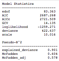
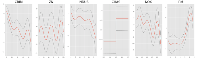
And we can similarly plot the feature dependencies:
XX = generate_X_grid(gam)
plt.rcParams['figure.figsize'] = (28, 8)
fig, axs = plt.subplots(1, len(boston.feature_names[0:6]))
titles = boston.feature_names
for i, ax in enumerate(axs):
    pdep, confi = gam.partial_dependence(XX, feature=i+1, width=.95)
    ax.plot(XX[:, i], pdep)
    ax.plot(XX[:, i], confi[0][:, 0], c='grey', ls='--')
    ax.plot(XX[:, i], confi[0][:, 1], c='grey', ls='--')
    ax.set_title(titles[i],fontsize=26)plt.show()
There are many more features and knobs to turn when building a GAM. Stay tuned for the advanced tutorial on further generalizing a GAM, CV for feature and smoothness selection, residual diagnostics, and more.
