Self-Driving Cars: Implementing Real-Time Traffic Light Detection and Classification in 2017
Today, basic traffic light detection is a solved problem. Innovations in deep learning and computer vision exist in the form of robust algorithms.
They work without developing code to manually determine the color, position, or location of the light. For example optimized R-CNN models can obtain state-of-the-art accuracy at real time speed.
So how does it work? Let’s explore and find some traffic lights!
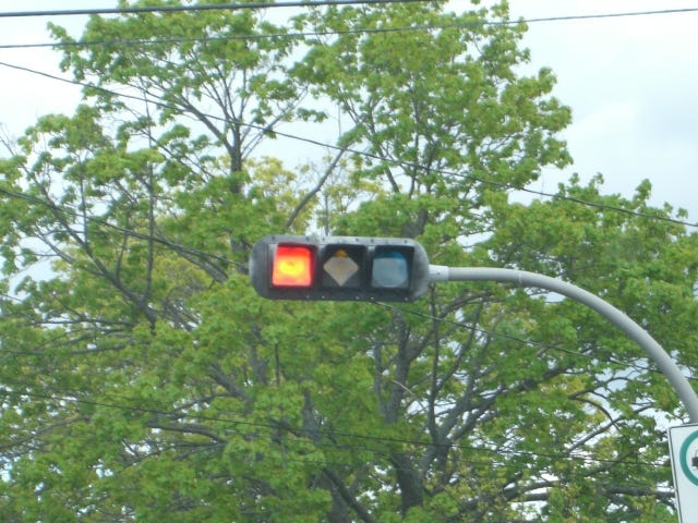
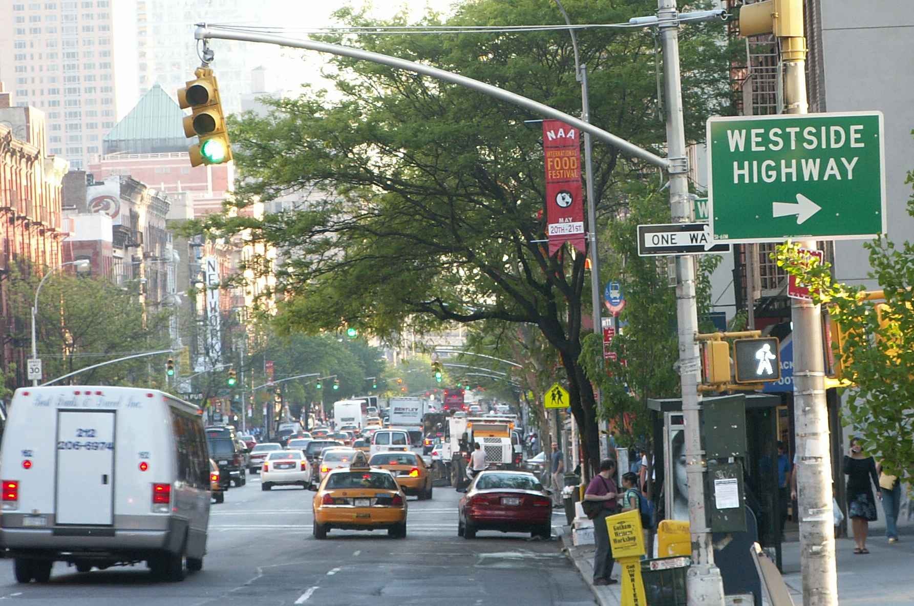
Quick, where are the traffic light(s)?
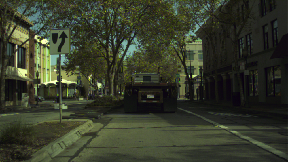

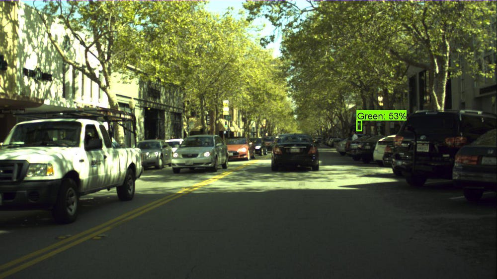
What the AI thinks:

Google’s approach, circa 2011
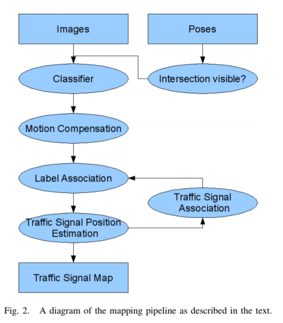
A team at Google used the approach of extracting the detected traffic light first, then running a second classifier on it. That approach provides flexibility; however, depending on the implementation it may come at the cost of added pipeline complexity and computation.
Perhaps more importantly it seems to rely on prior knowledge of expected traffic light locations. And more generally, doing classification as a second step adds a second network to train, test, etc.
Can it be done in one network, exclusively with an image and no prior information?
I first started by exploring Single Shot Detection (SSD) and ended up using Faster R-CNN due to it’s superior performance with small objects. I somewhat painfully recreated existing implementations to teach myself how it worked.
I then switched to using the open source tensorflow object detection api. This recently released toolset provides faster turnaround time for testing models and comes ready with popular pre-trained weights. It allowed me to focus more on the engineering implementation and less on the specifics of each neural network implementation.


In this paper they discuss performance trade offs of different approaches. For example, SSD (similar to YOLO) is great for medium to large objects, however fares significantly worse than Faster R-CNN for small objects. I confirmed this as in practice we had trouble getting SSD to converge well on the Bosch small traffic light dataset. In contrast, Faster R-CNN with Resnet got great results.
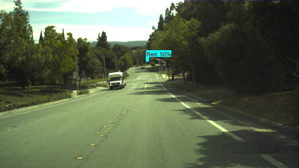
Want to see more? Check out the full videos: Test video. or Train video.
Adapting Bosch data for the Udacity self driving car
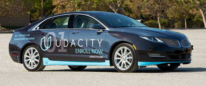
As part of a team of students from around the world we have been working on a limited test of a self driving car. On a tiny closed track the car must successfully follow a set of waypoints and identify a traffic light.
If you’re interested in the technical details check out our team’s code.
Double-transfer learning
We leaned heavily on transfer learning due to the limited amount of data available. The pipeline looks like this:
- COCO pre-trained network
- Bosch traffic light data
- Udacity real data (150 samples) or sim data (260 samples)
Using this method we got great results:
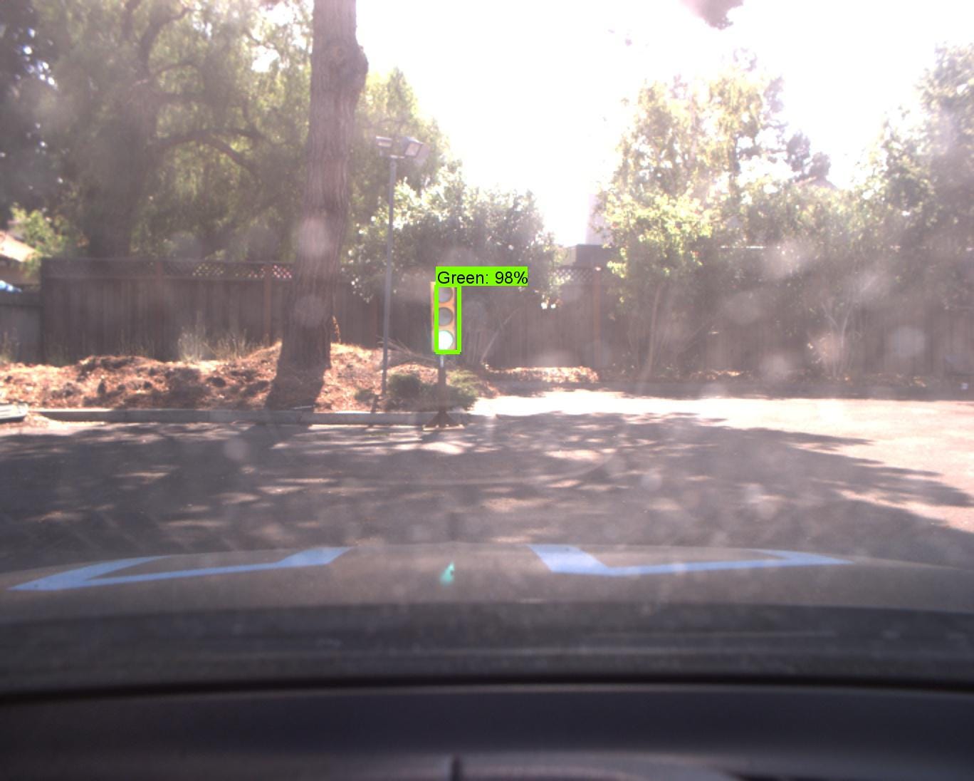
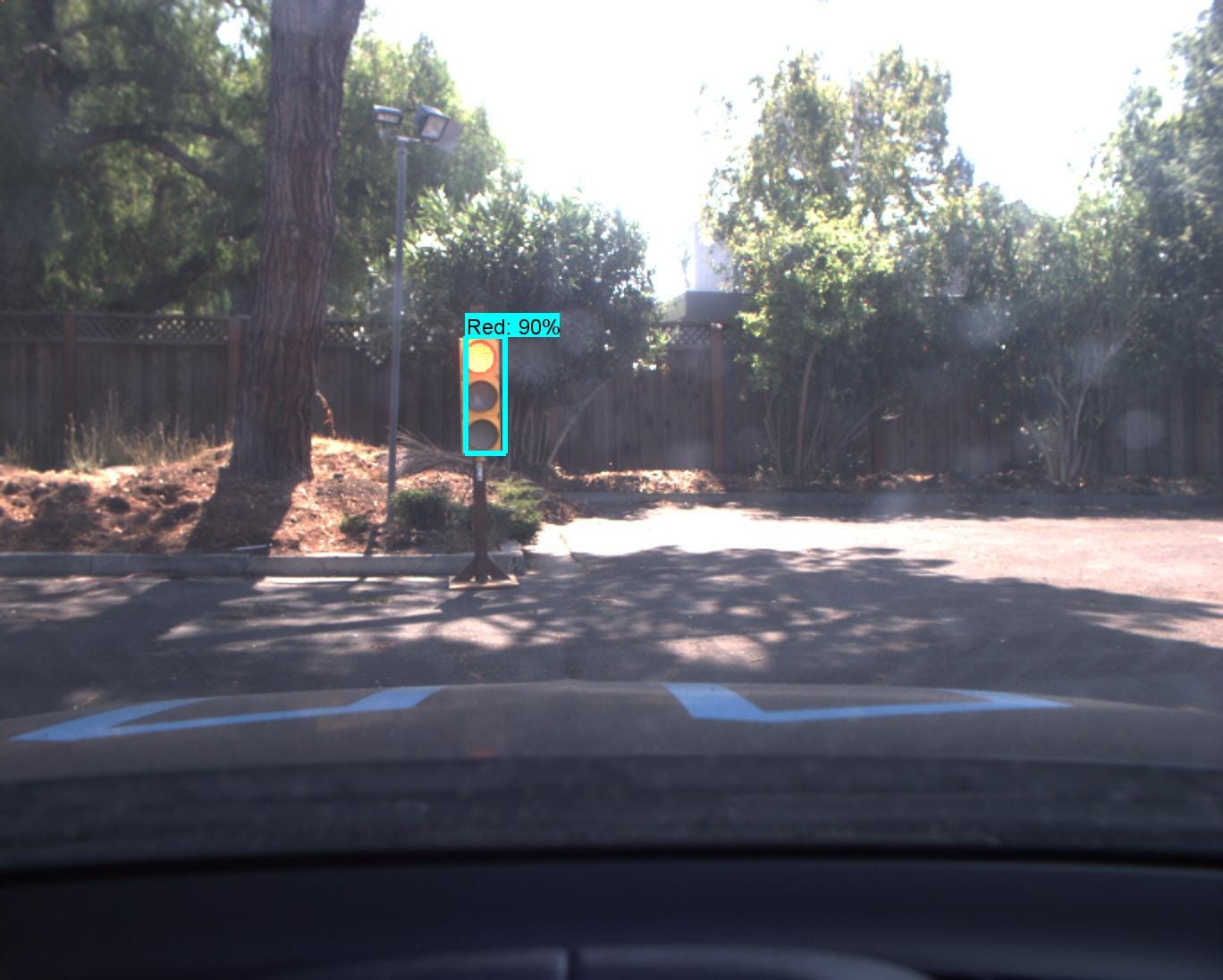
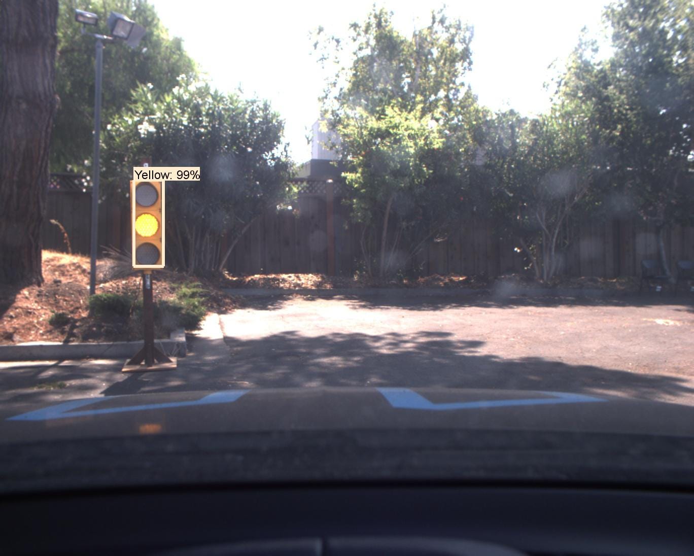
Why a deep learning based approach?
Traffic lights come in many different quantities, positions, shapes, sizes, and layouts. With a deep learning based approach these differences are “easy” — simply collect examples of the types of traffic lights in the area the car will be driving.

Motivation for high accuracy localization:
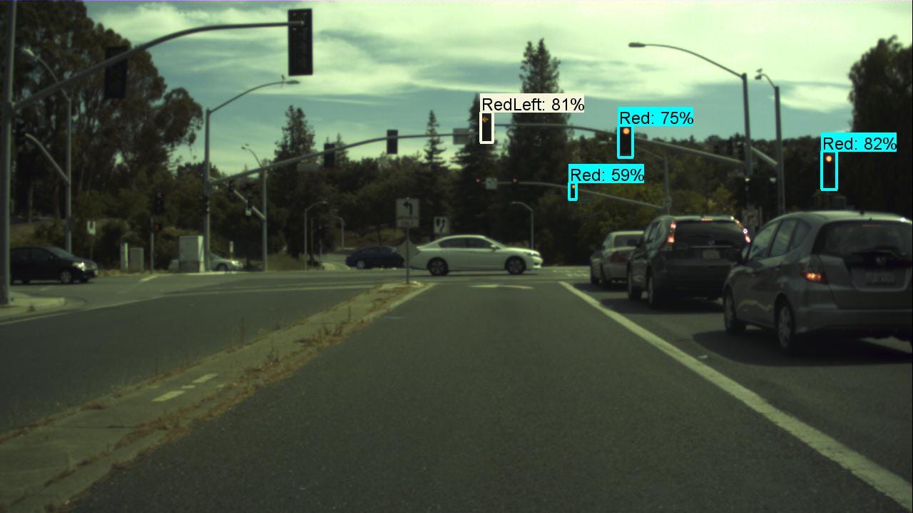
A high accuracy bounding box allows high accuracy distance estimation. The better the distance estimation, the closer we can match to other data points. For example, is a traffic light on the near side or far side of an intersection?
Real time performance (10+ Hz)
At first we were seeing inference times of around 220 ms. While this is fast compare to say a sliding window approach, I personally wouldn’t really consider 3–4 frames per second as real time.

Based on the papers suggestions we reduced the number of region proposals from the author’s original suggestion of 300, to 50.
This gave us a ~3x speed up in inference time. (~220 ms to ~80 ms) with similar accuracy.
This is predicting traffic lights that take up less than 1% of a 1280 x 720 image. For example in the above google paper they used images of 2040x1080 or 2.3x number of pixels.
Spectacular failure cases.
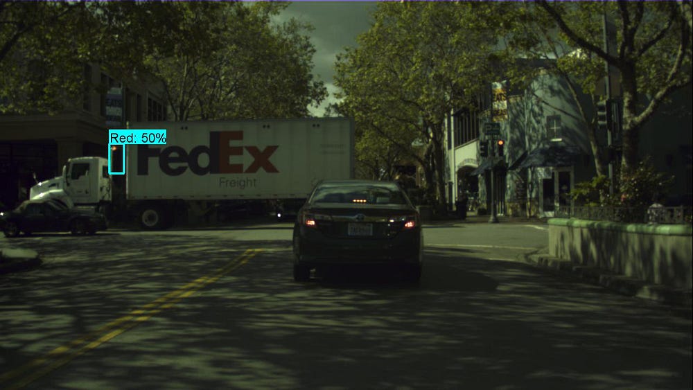
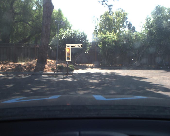
There are many examples where the system is not ready for production use. For example here it thinks it’s a yellow light!
That said, I can see many of these cases being overcome with more data, or simply more training. For example we trained to around 20,000 iterations, which is likely around 1/10 what’s needed for true convergence (ie most optimal model weight values).
One last thing

During testing I accidentally ran the network trained on simulated images (left) on real images.
Somehow it worked! And it worked well enough that it took a few odd failure cases to realize what was wrong!
Check out the results in this one example below:

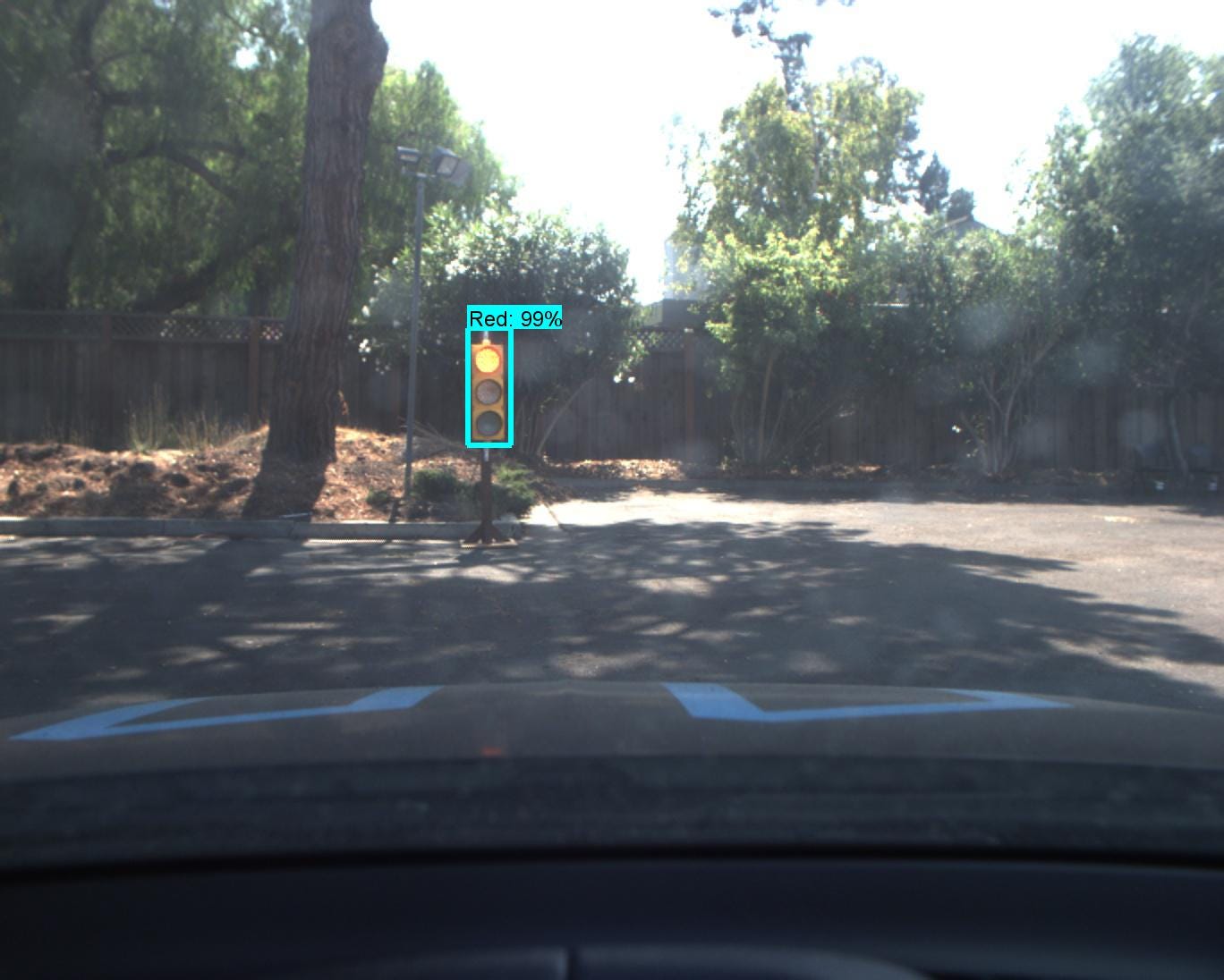
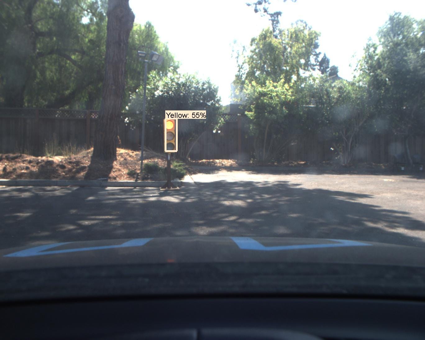
- Left: Bosch trained (different style of image) = no prediction over 50% confidence
- Center: Sim trained, (image above) = correct prediction
- Right: Real data trained (after bosch data) = incorrect prediction
It’s a reminder of an interesting opportunity. In theory, you could simulate any situation you wished, feed it to a deep learning system, and then have it generalize to a real life situation.
* Update Feb 2019 * If you are working on a deep learning system you may like Diffgram: Plug and play for computer vision!
Special thanks to Neil Hiddink and Cahya Ong for reviewing an earlier draft of this!
This is meant as a broad introductory exploration and it was not intended to be academically rigorous. Training was done without data augmentation (besides augmentation concepts inside the neural network itself and tensorflow object api), without dropout, etc. Ran on a GTX 1070 / Core i5. I used sloth to annotate the data.
Links summary:
- Deep learning code: https://github.com/swirlingsand/deeper-traffic-lights
- Self driving car code: https://github.com/nhiddink/SDCND_Capstone_TEC
- Test video: https://youtu.be/5e_9r9DROEY
- Train video: https://youtu.be/EN2jZ-9LRjs
