Neural networks for algorithmic trading. Volatility forecasting and custom loss functions
Hi again! In last three tutorials we compared different architectures for financial time series forecasting, realized how to do this forecasting adequately with correct data preprocessing and regularization and even did our forecasts based on multivariate time series. But there always stayed an important caveat — we were doing forecasting in terms of binary classification problem — asking if price will go up [1, 0] or down [0, 1] next day, and when we were switching to regression problem, e.g. forecasting the exact price, or percentage change of prices, we obtained horrible results, while binary classification showed 65% of accuracy. And of course, we would like to see nice plots where our forecast is gently and more or less correctly approximating actual results.
Previous posts:
- Simple time series forecasting (and mistakes done)
- Correct 1D time series forecasting + backtesting
- Multivariate time series forecasting
- Volatility forecasting and custom losses
- Multitask and multimodal learning
- Hyperparameters optimization
- Enhancing classical strategies with neural nets
- Probabilistic programming and Pyro forecasts
In this tutorial we will reconsider returns forecasting problem, design and check a new loss function for it, transforms returns into some sort of volatility and check different metrics for this problems as well. If you want to see the code first, check it out here.
Back to returns forecasting
First of all, let’s remember how we switch to returns (or percentage change) from original time series. I think, if we want to predict the return, we can switch all our dimensions (open, high, low, close, volume) to returns — they will be already normalized and this is more suitable option — having our input in form of returns if we plan to forecast return as well:
def data2change(data):
    change = pd.DataFrame(data).pct_change()
    change = change.replace([np.inf, -np.inf], np.nan)
    change = change.fillna(0.).values.tolist()
    return changeopenp = data_original.ix[:, 'Open'].tolist()
highp = data_original.ix[:, 'High'].tolist()
lowp = data_original.ix[:, 'Low'].tolist()
closep = data_original.ix[:, 'Adj Close'].tolist()
volumep = data_original.ix[:, 'Volume'].tolist()openp = data2change(openp)
highp = data2change(highp)
lowp = data2change(lowp)
closep = data2change(closep)
volumep = data2change(volumep)
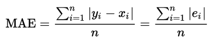
Let’s define the neural network as we usually do and ask it to minimize loss function, which we will choose for now as MAE — mean average error. It’s not the worst choice, especially taking into account, that in this case if we predict a percentage, we can easily report about, for instance, 5% of average error.
model = Sequential()
model.add(Convolution1D(input_shape = (WINDOW, EMB_SIZE),
                        nb_filter=16,
                        filter_length=4,
                        border_mode='same'))
model.add(MaxPooling1D(2))
model.add(LeakyReLU())
model.add(Convolution1D(nb_filter=32,
                        filter_length=4,
                        border_mode='same'))
model.add(MaxPooling1D(2))
model.add(LeakyReLU())
model.add(Flatten())model.add(Dense(16))
model.add(LeakyReLU())model.add(Dense(1))
model.add(Activation('linear'))opt = Nadam(lr=0.002)reduce_lr = ReduceLROnPlateau(monitor='val_loss', factor=0.9, patience=25, min_lr=0.000001, verbose=1)
checkpointer = ModelCheckpoint(filepath="lolkekr.hdf5", verbose=1, save_best_only=True)model.compile(optimizer=opt,
              loss='mae')history = model.fit(X_train, Y_train,
          nb_epoch = 100,
          batch_size = 128,
          verbose=1,
          validation_data=(X_test, Y_test),
          callbacks=[reduce_lr, checkpointer],
          shuffle=True)
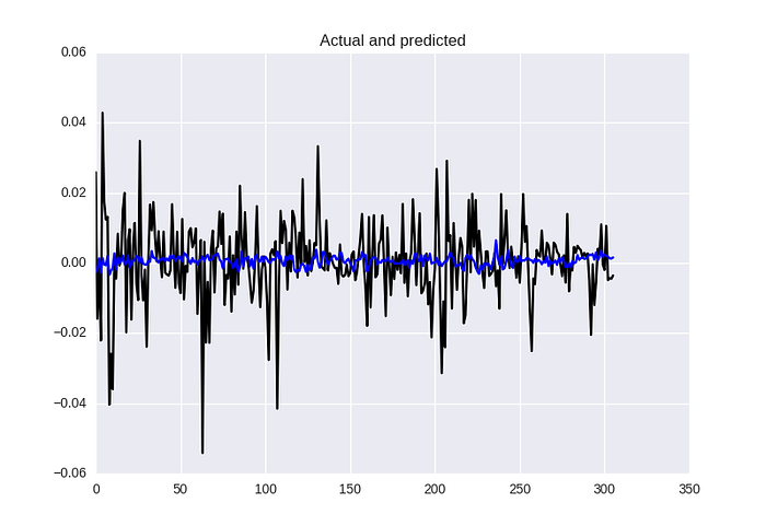
And we get following result:

In terms of different metrics we obtained MSE: 0.00013, MAE: 0.0082, MAPE: 144.4%.
Let’s look more close on MAE error:
And let’s remember what we were trying to predict before — how large and in what direction will be change. And now I want to ask you to read a small piece of text from amazing book about Bayesian methods:
Suppose the future return of a stock price is very small, say 0.01 (or 1%). We have a model that predicts the stock’s future price, and our profit and loss is directly tied to us acting on the prediction. How should we measure the loss associated with the model’s predictions, and subsequent future predictions? A squared-error loss is agnostic to the signage and would penalize a prediction of -0.01 equally as bad a prediction of 0.03. If you had made a bet based on your model’s prediction, you would have earned money with a prediction of 0.03, and lost money with a prediction of -0.01, yet our loss did not capture this. We need a better loss that takes into account the sign of the prediction and true value.
As we can see now, our current loss function MAE will not give us information about direction of change! We will try to fix it right now.
Returns with custom loss function
I would like to take a loss function from the book I have mentioned above and implement it for use in Keras:
def stock_loss(y_true, y_pred):
    alpha = 100.
    loss = K.switch(K.less(y_true * y_pred, 0), \
        alpha*y_pred**2 - K.sign(y_true)*y_pred + K.abs(y_true), \
        K.abs(y_true - y_pred)
        )
    return K.mean(loss, axis=-1)
While implementing “difficult” loss functions in Keras, take into account, that operations like “if-else-less-equal” and others have to be implemented with appropriate backend, for example, if-else block is implemented in my example with K.switch().
As we can see, if we forecast the direction (the sign) correctly, it’s same MAE (K.abs(y_true — y_pred)), but if not — we penalize our loss for the wrong sign (alpha*y_pred**2 — K.sign(y_true)*y_pred + K.abs(y_true)). Parameter alpha is needed to control the penalty amount. To apply this loss function to our model we need simply compile the model with it:
model.compile(optimizer=opt, loss=stock_loss)Let’s check results!
In terms of metrics it’s just slightly better: MSE 0.00013, MAE 0.0081 and MAPE 132%, but picture is still not satisfiable for out eyes, the model isn’t predicting power of fluctuation good enough (it’s a problem of a loss function, check the result in previous post, it’s not good as well, but look on the “size” of predictions!)
As an exercise, try to do the same trick — penalyzing loss function for wrong sign — but with MSE, because this loss function is more robust for regression problem.
Returns to volatility
First of all, we can all agree, that for this financial thing is very important to forecast when market will “jump”. Sometimes, it’s even not important what is the direction of jump — for example, in some young markets, like cryptocurrencies jumps almost always mean growth, or, for example, after large, but slow growing period the forecast of this jump most probably will mean some fall which will be a signal for us. In some sense, we are interested in forecasting the “variability” of prices in the future.
This amount of “variability” is called volatility (from Wikipedia):
In finance, volatility (symbol σ) is the degree of variation of a trading price series over time as measured by the standard deviation of logarithmic returns.
We will make this term a bit “dirtier” and will work with standard deviations of price returns over last N days and will try to predict how it will look for the next day.
volatility = []
for i in range(WINDOW, len(data)):
    window = highp[i-WINDOW:i]
    volatility.append(np.std(window))
The plot of these “monthly volatilities” for our GOOGL stock will look like this:
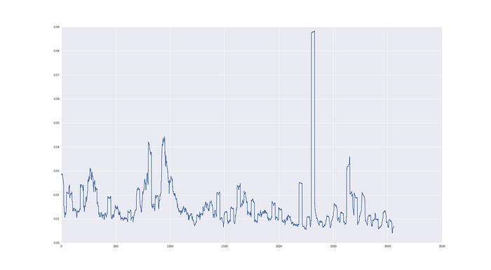
And let’s check, how we can forecast this quantity!
Volatility forecasting
The data preparation process can look like:
for i in range(0, len(data_original), STEP):
    try:
        o = openp[i:i+WINDOW]
        h = highp[i:i+WINDOW]
        l = lowp[i:i+WINDOW]
        c = closep[i:i+WINDOW]
        v = volumep[i:i+WINDOW]
        volat = volatility[i:i+WINDOW]        y_i = volatility[i+WINDOW+FORECAST]
        x_i = np.column_stack((volat, o, h, l, c, v))
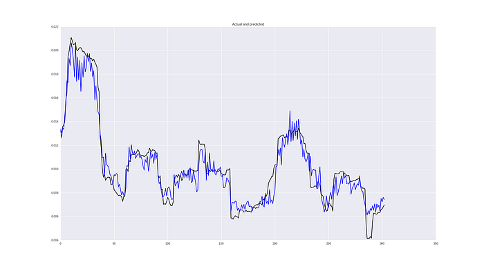
We will take the same neural network architecture as above, change the loss function MSE and repeat the process for forecasting the volatility. The result will look like:
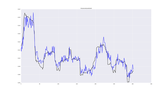
In general, it looks not bad at all! Of course, some jumps are predicted too late, but in general ability to catch dependencies is good! In terms of metrics it’s MSE 2.5426229985e-05, MAE 0.0037 and 38% of MAPE.
I also would like to encourage you to try different loss functions for volatility, for example from this presentation. For example, let’s try with MSE log:
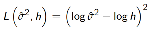
def mse_log(y_true, y_pred):
    y_pred = K.clip(y_pred, epsilon, 1.0 - epsilon)
    loss = K.square(K.log(y_true) - K.log(y_pred))
    return K.mean(loss, axis=-1)model.compile(optimizer=opt, loss=mse_log)
Result looks like:
Metrics are MSE 2.52380132336e-05, MAE 0.0037 and MAPE 37%. Not that much, but already better! Some other loss functions you can find implemented in repository.
Conclusions
In this tutorial I tried to show several very important moments in time series forecasting:
- While having a general goal for forecasting financial time series, we can transform our data in different way in order to work with better time series — we couldn’t work adequately with prices and returns, but forecasting variability of returns works not bad at all!
- You have to design loss functions very carefully depending on the problem and check different hypothesis. For returns giving a penalty for wrong sign is good idea, MSE on log values is better for volatility.
Don’t forget, that these ideas you can apply to different problems related to predictive analytics based on time series.
In next tutorials we will design and test more complicated and different hypotheses from neural networks world, so stay tuned!
P.S.
Follow me also in Facebook for AI articles that are too short for Medium, Instagram for personal stuff and Linkedin!

